11  Measurement Error

11.1 Introduction

Measurement error in the dependent variable inflates standard errors. But the OLS estimator is still BLUE. The same cannot be said of measurement error in the independent variable. It will produce a correlation between \(X\) and \(\epsilon\), which will bias the parameter estimates.

11.2 Measurement Error in the Dependent Variable

In the dependent variable, we’ll generally observe greater variance estimates. Let the true data-generating process be

\[Y^{*}_i = \alpha + \beta X_i + \epsilon_i\]

But let’s assume we cannot observe the true \(Y^{*}\), and instead observe \(Y_i\) with some degree of error,

\[Y_i = Y^{*}_i + u_i.\]

Then,

\[Y_i = \alpha + \beta X_i + \epsilon_i + u_i,\]

where there are now two error components. The variance of the slope estimator becomes

\[\text{var}(b) = \frac{\sigma^2_u + \sigma^2_{\epsilon}}{\sum (X_i - \bar{X})^2}.\]

As measurement error decreases (i.e., \(\sigma^2_u\) decreases), so too will the standard errors associated with \(b\). Importantly, the expected value of \(b\) is unchanged – the estimator is still unbiased, provided \(u_i\) is uncorrelated with \(X_i\).

11.3 Measurement Error in the Independent Variable

On the other hand, for the independent variable(s), assume the true model is

\[Y_i = \alpha + \beta X_i^{*} + \epsilon_i.\]

But assume we cannot observe the true \(X^{*}\), and instead observe \(X_i\) with some degree of error,

\[X_i = X^{*}_i + \gamma_i.\]

Substituting \(X^{*}_i = X_i - \gamma_i\),

\[Y_i = \alpha + \beta X_i + \epsilon_i - \beta \gamma_i.\]

Call the combined error components \(z_i = \epsilon_i - \beta \gamma_i\). Now the regressor and the composite error are correlated:

\[\text{cov}(X, z) = -\beta \, \sigma^2_{\gamma}.\]

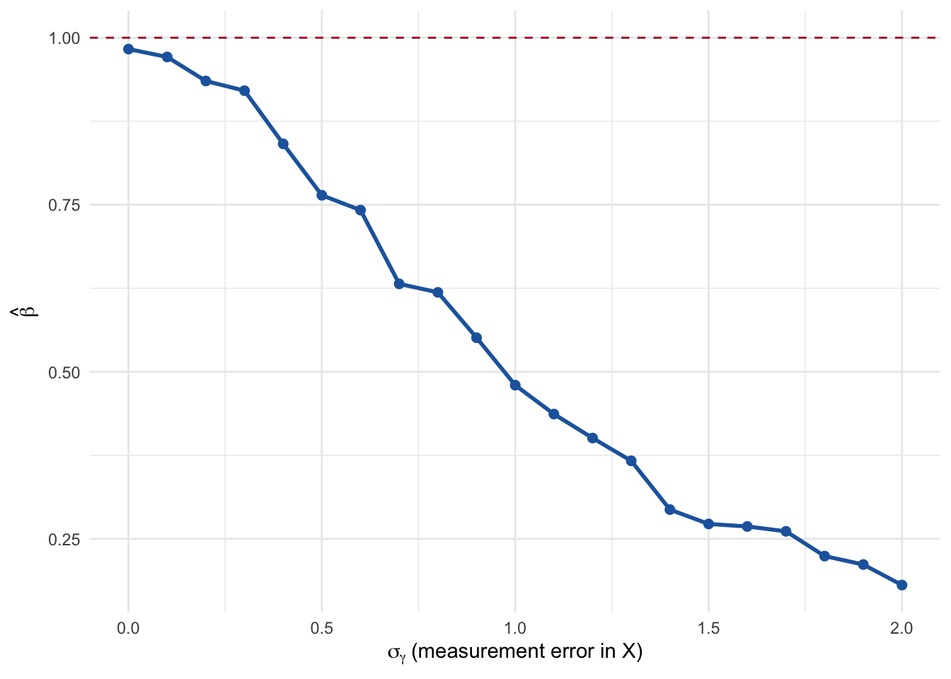
As measurement error increases, the magnitude of the estimated coefficient for \(\beta\) will shrink toward zero. Measurement error in the independent variable produces an attenuation bias.

With measurement error in the IV(s), OLS is biased. With measurement error in the DV, OLS is BLUE, but standard errors will be larger. (Recall the bias–variance tradeoff.)

11.4 Simulation: Attenuation Bias

Let’s see attenuation bias in action. We’ll simulate a true \(X^{*}\), generate \(Y\) from the true model, and then estimate \(\beta\) using progressively noisier measures of \(X\).

set.seed(2026)
n <- 1000
beta_true <- 1.0

x_star  <- rnorm(n, 0, 1)
epsilon <- rnorm(n, 0, 1)
y       <- 0 + beta_true * x_star + epsilon

sigma_gamma_grid <- seq(0, 2, by = 0.1)

results <- data.frame(
  sigma_gamma = sigma_gamma_grid,
  beta_hat    = NA_real_
)

for (i in seq_along(sigma_gamma_grid)) {
  sg <- sigma_gamma_grid[i]
  x_obs <- x_star + rnorm(n, 0, sg)
  results$beta_hat[i] <- coef(lm(y ~ x_obs))[2]
}

ggplot(results, aes(x = sigma_gamma, y = beta_hat)) +
  geom_hline(yintercept = beta_true, linetype = "dashed", color = az_red) +
  geom_line(color = az_blue, linewidth = 1) +
  geom_point(color = az_blue, size = 2) +
  labs(
    x = expression(sigma[gamma] ~ "(measurement error in X)"),
    y = expression(hat(beta))
  ) +
  theme_minimal()

Figure 11.1: Attenuation bias: as measurement error in X increases, the estimated slope shrinks toward zero. The dashed line is the true β = 1.

The theoretical result is that, with classical measurement error, the probability limit of the OLS slope is

\[\text{plim} \, \hat{\beta} = \beta \cdot \frac{\sigma^2_{X^{*}}}{\sigma^2_{X^{*}} + \sigma^2_{\gamma}}.\]

The term \(\sigma^2_{X^{*}} / (\sigma^2_{X^{*}} + \sigma^2_{\gamma})\) is sometimes called the reliability of \(X\) and lies in \([0, 1]\). As \(\sigma^2_{\gamma} \to 0\), reliability approaches 1 and \(\hat{\beta}\) approaches \(\beta\). As \(\sigma^2_{\gamma}\) grows, reliability – and \(\hat{\beta}\) – shrinks toward zero.

11.5 Simulation: Measurement Error in Y

In contrast, measurement error in \(Y\) leaves the point estimate alone (on average) and simply inflates the standard error.

Table 11.1

set.seed(2026)
n <- 500
x <- rnorm(n, 0, 1)
y_star <- 0 + 1 * x + rnorm(n, 0, 1)

sigma_u_grid <- c(0, 0.5, 1, 2, 4)

me_dv <- lapply(sigma_u_grid, function(su) {
  y_obs <- y_star + rnorm(n, 0, su)
  fit   <- lm(y_obs ~ x)
  data.frame(
    sigma_u = su,
    beta_hat = coef(fit)[2],
    se_beta  = sqrt(diag(vcov(fit)))[2]
  )
}) |> do.call(rbind, args = _)

me_dv

   sigma_u  beta_hat    se_beta
x      0.0 0.9790198 0.04183781
x1     0.5 0.9857252 0.04663237
x2     1.0 1.0047861 0.05659268
x3     2.0 0.9722704 0.09442010
x4     4.0 0.9719465 0.18148846

Coefficients hover around the true value of \(1\); standard errors grow roughly with \(\sigma_u\).

11.6 Corrections

Many methods are available to correct for measurement error – most are outside the scope of this class, but they include:

• Factor analysis and structural equation models that explicitly model a latent construct separate from its indicators.
• Multi-item scales, which rely on true-score theory. Averaging several noisy indicators of the same construct reduces the measurement-error variance roughly by a factor of \(1/k\).
• Item response theory, which models the relationship between a latent trait and discrete responses.
• Two-stage least squares (instrumental variables), where an instrument correlated with \(X^{*}\) but uncorrelated with \(\gamma\) and \(\epsilon\) can recover a consistent estimate of \(\beta\).

One should always strive to measure constructs with as much accuracy as possible, particularly if the noisy variable is a covariate rather than the outcome. And – always – check for coding errors.